Excel Figures with Directional Arrows

I needed streamlines and a I wanted arrows to show the flow direction of the flow.

I scoured the web and didn't find a single solution but I did find the pieces I needed to make an VBA macro to add directional arrows to my streamlines

Here's the instructions

Pull in your Original XY Data in the Original Sheet - I use the Matlab code below to generate constant streamlines

In the Control sheet, enter the number of points before an arrowhead is drawn in the appropriate cell
This sets the distance between arrowheads

Click Parse Data
This will take the original data and break it up into many different columns that can be added as individual series

Click on the figure in the Figure sheet
This is a prerequisite for the next step

From the XL toolbox addon, click Chart series>Add Many Series
Select all the cells containing the data and labels for the series from the Parsed for Streamlines sheet

Change the chart type to XYScatterSmoothNoMarkers

Select Individual X values/labels for each series

click Add series
This adds all the new XY pairs as individual series in the figure

Once it's completed, the Format Chart Series button can be used to automatically format the chart.
This automatically adds arrowheads and sets the formatting of the data series.   Since there will be A LOT of series, this is a life saver.  The drawback of this operation is that it you have to edit the VBA code to change the automatic formatting properties.


Figure Generator

Matlab Streamline Code

XL Toolbox "Cannot find object"

On my laptop with Office 2010, I get an error every time I install/update Daniel's XL toolbox.  It says something like "object cannot be found..."

From the forums,
http://xltoolbox.sourceforge.net/referencesfix/
it says to uncheck any references listed as "missing."  I have none.  What seems to work though is simply saving the macro.

In excel hit alt+F11 to open the macro editor.  Highlight Daniel's XL toolbox in the tree.  Click the save button.  That's it.

The first time I had this happen, I spend hour(s) trying to find the solution and ended up finding a forum that had me delete something out of the tree and saving...it worked but I can't find the forum.  It was supposed to rebuild something in the macro and save it.  Since I saved it, it might have been the only key.

Publication Quality Legends in Excel

I've already written about making publication quality figures in excel.  The legends still cause problem since you can't edit individual characters.

For instance, if I have a legend label z = 0, "z" needs to be italics since it's a variable.  I can only italic the entire entry "z=0".  This is incorrect since the "0" shouldn't be italic.

The quick and dirty answer is to insert a text box and set the correct legend entries there, then move it over the top of the original entries to cover them up.  EXCEPT, you can adjust the size of the legend causing the spacing between entries to also adjust, but you can't adjust the spacing in a text box.  For me, I run the risk of running out of real estate on the figure because I can't make the legend smaller than the text box.

I have mathtype (this may work in equation editor too) so what I've done is typeset the legend entries in mathtype and copy them to the excel figure one at a time.  Make sure you have the cut and copy preferences set to MathML or LaTeX or else they won't embed into the figure and therefore, won't copy to word as an excel object (exporting as image should work though).

If you have your figure set up like I do in my previous post and the cut and copy preferences set, then each mathtype equation will show up as a picture.  For equations without subscripts and superscripts, setting the picture height to 0.16 will make the text 9 point - which is what I use for figures and captions.  Equations with Subscripts and Superscripts or fractions may have to be adjusted differently.

Once I have all the labels inserted, I align and group them and set the background to white.

Other plotting software can handle individual characters in legends.  Excel should be able to as well.

Publication Quality Figures in Excel

Whoever at Microsoft thought that the cartoon-ish format defaults for Excel graphs clearly doesn't understand the professionalism required for journal quality figures.  It's actually so bad that when I see scientific data presented in default Excel graphs, I instantly begin to question the validity of the work.  If anyone at Microsoft happens to read this post, please do some homework and compare the quality of Excel figures to let's say OriginLab or GraphPad.

Besides the visuals, Excel also needs to be able to export figures at fixed dimensions as a variety of formats.  PNG is probably the most viable since it works with both word documents and PDFLaTeX.

Fortunately, all hope is not lost.  Many of us have access to Excel but not other graphing programs (cost!).  Follow along and before you know it, your figures will be publication worthy!

First off, you'll need the free add-on Daniel's XL Toolbox http://xltoolbox.sourceforge.net/ This add-on allows for export of high quality figures with set dimensions with a variety of formats.  Great Job on this addon!

Download my template.  Click on the link.  Then in the new window select File>Download or click the down arrow button at the top left.

You can replace the data and the figure will automatically update itself.  A couple key tricks:

1)  Format Chart Area and fix the height and width.  I prefer 1.8 x 3" for fitting two figures side by side.
2)  Everything needs to be black and white (or grayscale if acceptable)
3)  I prefer time new roman for the font 10 pts
4)  Axis titles are italicized (any variable is italicized)
5)  The real trick is making sure everything lines up
 - Notice the cells behind the figure are very small.  Under chart tools>Format>Align select snap to grid.  Now when you drag an axis or label, it will always snap the the cell boundaries.  The smaller the cells, the more control over positioning.

This will get you started.  If you're starting from scratch, you'll most likely have to set the line width for the axis and data.

Once you're happy with the figure, click XL Toolbox>Export>Export for publication. Select the format and check the height and width.  This often isn't correct.  I don't know if this is a bug or what.  To fix it:  go back to the figure go to Format Chart Area>Size and click Lock Aspect Ratio.  Sometimes when it's locked you'll need to unlock it, sometimes when it's unlocked you'll need to lock it.  Either way, this fixes things.

Here's the final product

Update:  Use 1000dpi and use the PRINT and select Adobe PDF command from Word or else the images seem to be downgraded.  I used the max dpi (2400) and it couldn't handle it in Word 2013.

Hyperlink Combo Boxes in Excel with VBA

There is a lot of forums about how to do this and the best I've seen is using named ranges and data validation lists. I think there is a better way.

Problem: I want to make a drop down menu with hyperlinks to other worksheets

Solution: Write a simple VBA macro (I promise, it's really easy!)

Step 1: Make sure all your worksheets are cleanly titled. If you have several distinct groups of worksheets, then the first word of the title should be the same for the group. In this example, I have several worksheets grouped in "Tournament" so my titles are like "Tournament Setup", "Tournament Registration" etc.

Step 2: Create a worksheet to house all the menu options. This is not necessary if you can efficiently generate list items from the original worksheets. For example purposes, we will keep all our entries here. Also, if you want the code to work as shown below follow these steps exactly and name this sheet NavMenu.

Step 3: Designate a column for the menu items. If you want the code provided to work without modifying the cell locations, then the sheet should be built like

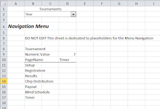
Cells B11:B17 are the menu items. For now, just type in the menu items in this range. The menu items should NOT include the group label. This will be added automatically in the code. Cell B8 is the group label. You can go ahead and add this too.

Step 4: Create a form control combobox (not activeX). Right click and click format control. In Input Range select the range containing the menu items. Here it is NavMenu!$B$11:$B$18. I include Cell B18 so I have a blank item to rest the menu to. You'll see what i mean below.

In the cell link box enter NavMenu!$D$9. It is important to specify the NavMenu worksheet since you'll use this on many pages and it must only modify the cells in the NavMenu worksheet, not the current sheet. Now you should have a combo box that contains all the menu items and posts the index in cell D9.

Step 5: Cell D10 is the name of the menu item. To do this we use the offset command. In Cell D10 enter =OFFSET(B8,D9+2,0,,) . This takes B8 as the reference cell, counts value(D9)+2 rows down, and displays whatever is in that cell. In our case, it's the menu item name.

Step 6: In Cell D8 enter =COUNTA(B11:B18). This is not shown in the picture above because i just added it. It counts the total number of non blank cells in the range. I include B18 because when I insert new item, the range will automatically adjust. New items are inserted in the menu by insert (shift cells down) at B18.

Step 7: Open up the Developer menu (search google if it's not already displayed in your ribbon) and visual basic. Create a new module for the menu and paste:

Sub TournamentMenu()

Dim PageName As String, GroupName As String, SheetName As String

Dim ItemNum As Integer

ItemNum = ['NavMenu'!D8] 'number of menu items

PageName = ['NavMenu'!D10] 'page name

GroupName = ['NavMenu'!B8] 'group name

If PageName = "0" Then 'condition to exit if blank

Exit Sub

End If

SheetName = GroupName & " " & PageName 'join the groupname and pagename

Sheets(SheetName).Select 'navigate to the sheet

['NavMenu'!D9] = ItemNum + 1 'reset the menu to the blank entry

End Sub

Step 8: Right click on the combobox and click assign macro. Select TournamentMenu and you're done!

Repeat for different menus. Modify the cell locations for ItemNum PageName and GroupName for each menu.

Generating Unique Random Numbers in VBA Excel

Problem: Generate a list of unique random integers between two bounds in VBA and Excel

Solution: I started with the code from here. The original code output the random numbers as a string residing within the same cell. Needed each random number to appear in its own cell. The context was to randomize seating for a poker game, hence the variable names players

I pull the input data from the excel cells directly so adjust your code to match the cells you want to input:

Top - upper bound

Bottom - lower bound

Players - cell range of players (The range of cells next to the list of player where each player name is located in a column of cells)

Execute code on button click

Sub Seating()

Dim iArr As Variant

Dim i As Integer

Dim r As Integer

Dim Top As Integer

Dim Bottom As Integer

Dim temp As Integer

Dim Players As Range, Cell As Object

Set Players = Range("W10:W25")

Top = [V7]

Bottom = 1

Application.Volatile

ReDim iArr(Bottom To Top)

For i = Bottom To Top

iArr(i) = i

Next i

For i = Top To Bottom + 1 Step -1

r = Int(Rnd() * (i - Bottom + 1)) + Bottom

temp = iArr(r)

iArr(r) = iArr(i)

iArr(i) = temp

Next i

j = 1

For Each Cell In Players

Cell = iArr(j)

j = j + 1

If j > Top Then

Exit For

End If

Next

End Sub